Towards Certified Digital Audio Processing
Emilio Jesús Gallego Arias
(joint work with Pierre Jouvelot)
MINES ParisTech, PSL Research University, France
December 5th 2016 - Synchron 2016 - Bamberg
FEEVER ANR Project
Real Time Signal Processing
$\cap$
Programming Language Theory
$\cap$
Theorem Proving
Key Goal: Arbitrary Formal Proofs
- Linearity: A set of programs correspond to an LTI system.
- Simulation: Different executions/implementations denote the same program. Including compilation!
- Approximation: A program approximates another program or mathematical system. Quite free-form! Think of relating a program to its Z-transform.
Basic Audio Objects
Recursive 2nd order Filter
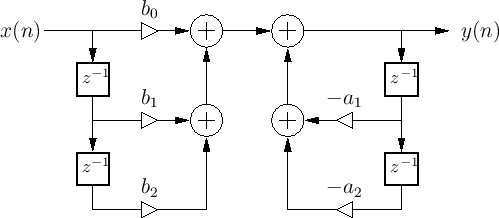
Image Credits: Julius Orion Smith III
Wave-guide Resonator
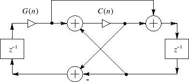
Image Credits: Julius Orion Smith III
Programs correspond to synchronous data-flow.
A Theorem Road-map
Julius Orion Smith III audio-focused book's series:
- Mathematics of the Discrete Fourier Transform (DFT) [Partially handled + missing inf. sum.]
- Introduction to Digital Filters [Work of this talk]
- Physical Audio Signal Processing [Minor bits in this talk + missing ODE]
- Spectral Audio Signal Processing [Future work]
Main Relevant Points:
- Free mix of mathematics and computation.
- Linear algebra is pervasive.
- Proofs of uneven difficulty, not constructive-friendly.
Where to Look?
VeriDrone Project[Ricketts, Machela, Lerner, ...]
[EMSOFT 2016] traces+LTL, continuity, Lyapunov.
Lustre Certified Compiler[Bourke et al.]
Work in progress, denotational semantics?
FRP/Arrows[Krishnaswami, Elliot, Hughes, Hudak, Nilsson, ...]
Nice functional PL techniques; too abstract for real-time sample-based DSP.
Synchronous Languages [Berry, Caspi, Halbwachs, Pouzet, Guatto, ...]
Guatto's PhD Most related to our approach.
Suited to linear algebra/DSP?
Data-intensive vs control-intensive require quite
different control techniques. [Berry, 2000]
Isabelle/HOL[Akbarpour, Tahar et al.]
Fixed systems, numerical issues.
The Plan
Formal Proof and Semantics
$$ \forall p, ⟦p⟧_A = ⟦T(p)⟧_B $$Main question, what is ⟦ ⟧?
Borrow Techniques from Functional Programming to Attack the Problem:
- Define a functional, dataflow-like language.
- Untyped operational semantics!
- Classify well-behaved programs wrt the enviroment.
- Logical Relations
- ?
- Profit!
What now: Pre-Wagner
Simple λ-calculus with feedback, pre, and stable types.
Types and Syntax:
Pre-Wagner: Op. Semantics
Assume causal feedback. Big-step, time-indexed relation. Every program reduces to a value at time step $n$. Similar to synchronous data-flow.
Examples: DF-I Filter
Note size polymorphism of the dot operator:
Examples: DF-II
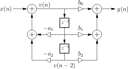
Compare with df1:
Examples: Wave-Guide OSC
we write $x' \equiv \fpre{x}{1}, y' \equiv \fpre{y}{1}$. With different sugar:
Towards a New Semantics Or some critics of "pre"
A) Compare a typical FIR:
$$ x \cdot y ≡ \sum_i x[i] ⬝ \fpre{y}{i} \qquad \text{vs} \qquad x \cdot y ≡ \sum_i x[i] ⬝ y[i] $$- Model where pre behaves like array indexing?
B) Evaluation strategy and caching?
$$ \begin{array}{ll} \text{collect} &: R ⊗ \dots ⊗ R ⇒_0 R \\ \text{avg} &: R ⇒_{100} R \\ \text{process} &: R ⊗ \dots ⊗ R ⇒_? R \\ \text{process} &= avg ∘ collect \end{array} $$What should be the type of $\text{process}$ ? A caching of 100? Ups!
C) How can we drop the causality requirement? "pre" doesn't need it!
Val-Wagner
Assume CBV, only variables can be time-addressed:
Types and Syntax:
Where is my Pre?
Variables are arrays with history; we recover "pre" by "eta":
Untyped Operational Semantics using a stack of arrays ${\cal E}$:
Feedback is interpreted now by "sequential" execution! We allow it to update the environment. We can alternatively replace $ε$ for $\vec{0}$.
Interaction and Typing
Environment ${\cal E}$ interacts well with $e$ if it contains enough history.
Type System:
Co-effects keep track of history-access. Array subtyping and polarity (optional):
Main Lemma:
If $Γ_\vm ⊢ e : T$ and $Γ_\vm \vdash {\cal E}$ and $e$ is causal (definition of your choice!) then $$ ∀ n. {\cal E}~ \bot_n~ e \qquad \qquad \qquad (\equiv {\cal E}~ \bot~ e) $$
Semantics for types $⟦T⟧$: sets closed under $⊥$.
Case Study I: Linearity
We characterize the set of linear Wagner programs, a first step for the Z-transform theory of linear programs.
Addition of programs:
Lin-Wagner is obtained by dropping constants and non-linear operations. What is the right definition of linearity? We use a logical relation:
The relation is simple, but works at higher-types. Every Lin-Wagner program satisfies the relation! The proof proceeds, first, by induction on the typing derivation, then by induction on the number of steps.
Case Study I: Linearity
What about multi-linearity? A brief comment:
Compare: $$ \begin{array}{l} λ x. Λ y . x \cdot y : R → S ⇒ T \\ Λ x. Λ y . x \cdot y : R ⇒ S ⇒ T \end{array} $$
Case Study II: The SSSM Abstract Machine
Lin/Val-Wagner semantics compute the full history of the argument at each function call. We introduce a heap and define a monadic semantics for types:
The binary heap follows the structure of expressions.
Case Study II: The SSSM Abstract Machine
Evaluation as usual. Operations to "focus" the heap, add a new value, etc...
Idea: put/get respect initial buffer size.
Case Study II: The SSSM Abstract Machine
A well-formed heap for that program contains the proper amount of buffering for $e$, plus the correct values for the past. The main lemma is then:
$$ {\cal E} ≈_n ({\cal D, H}) → ⟨ {\cal E} ∥ e ⟩_{n+1} = \mathsf{exprV~{\cal D}~e}~H $$
Case Study III: Frequency Domain
Quick Review:
- Frequency Response = impulse response output.
- A filter is stable = its Frequency Response is summable.
- Stability implied by the existence of the DTFT.
- The DFT may approximate the DTFT.
- The DTFT is the evaluation of the Z-transform for the unit circle.
Current state:
- Previous linearity theorem and a notion of DFT in Coq are prerequisites.
- Work in progress, Z-semantics defined propositionaly.
- Requires a representation theorem to interpret types.
Conclusions
- Long path, technique is powerful. Applications to other areas, extensions (references, polymorphism).
- Multirate/clocks: Very simple reclocking primitives, enough for our needs. Better support under study.
- Some other limitations: false cycle circuits.
- Implementation in Ocaml with a core type system. Interesting design space, in particular wrt to closures.
- Coq formalization: working but more experience is needed to decide on some implementation details.
- Connection to State Space analysis, control theory, MIMO systems.
- Floating Point Interpretation. Numerical issues are pervasive in this domain, but trying to get there.
- Verification of program and transform optimization. [Püschel]
Thanks!

The fun starts !!
We embed Val-Wagner into Coq using a lightweight dependenly typed syntax. We focus on a reduced subset, leaving higher order, rates, and stable values for later. Recall that: $ R ⇒ R ⇒ R ≈ R ⊗ R → R $. Thus:
Program Interpreation:
The lightly-typed syntax allows to overcome typical termination issues in our embedding and provide an "executable" semantics inside Coq, we want something like:
We take a simple choice and use $\mathsf{env} = \mathsf{seq}~(\mathsf{seq}~ℝ)$. For type interpretation we use:
Thus functions have access to all history. We also provide an initial value for every type. Many more refinements are possible!
Step-Indexing
The definition of step-indexing in Coq is tricky, interpretation proceeds by induction on time and expressions. We must use a stronger induction principle for Coq to be happy:
Geometric Signal Theory
The DFT:
$$ X(\omega_k) = \ip{x^T, \omega_k} ~~\text{where}~~ \omega_k = \omega^{k*0},\ldots,\omega^{k*(N-1)} $$Most properties are an immediate consequency of matrix multiplication lemmas in math-comp.
In matrix form:
Primitive roots:
The constructive algebraic numbers in mathcomp provides us with a primitive root of the unity such that $ω^N = 1$.
In an Ideal World...
... we'd have everything we need in our library.
- We are not so far from it.
- Took the definitions from classfun.v and proved:
Energy theorems are easy corollaries. Compact development for now, see the library.
Transfer Function:
We now want to relate our programs to their transfer function. The first step is to define the Z-interpreation for types:
We'd like a theorem relating the summability of:
to the evaluation of the transfer function. We can establish:
Z-Interpretation of Programs
It is work in progress; we tried to build an effective procedure, it is difficult.
Current approach: We use a relation
First Try: Mini-Faust [LAC2015]
- Faust [Orlarey 2002]: DSL for DSP arrow-like, point-free combinators.
- Coq semantics: step-indexing, math-comp.
- Define a (sample-based) logic for reasoning about this programs.
Problems with the approach:
- DSP not friendly to point-free combinators (matrices).
- PL methods awkward for DSP experts.
- Doesn't work well for complex examples.
- Key point for proofs: Semantics of programs.
Executing Equations:
This system is simple but convenient due to its natural, computable, and canonical embedding, what can be done in the case of Lustre-like equations?
A possible roadmap:
- Define a topological type $\mathsf{ts}$ and sort function $\mathsf{topo : eqn \to option~ ts}$, from sets of equations to schedules.
- Define an interpreter for $\mathsf{ts}$.
- [Optional]: If the program is well-clocked, then $\mathsf{topo}$ succeeds. Prove a): Prove topo is sound (the output respects the original eqn).
- Prove b): All possible schedules return the same value in the interpreter. (invariance under permutation)
- The rest of the proof should be "free" of scheduling choices. The intrepreter should expose the internal state from the begining.
Handling Clocked Streams
[The beginning of it all]
Port of the Lucid paper to Coq/Ssreflect; replace dependently typed streams by sequences plus a decidable well-clocked relation:
Decidability provides "inversion views" (also called small inversion sometimes) which are very convenient.
Example: Filter Stability
$$ \fjud{\fpo}{f}{\fpw} \iff \forall t, \fpo(i(t)) \Rightarrow \fpw(f(i)(t)) $$In PL terms: $ \fjud{x \in [a,b]}{\mathsf{*(1-c) : + \sim *(c)}}{x \in [a,b]} $
In DSP terms: The impulse response decays to 0 as time goes to infinity.
- Higher-order filters may make PL methods impractical.
- State seen as matrices/arrays.
Context of the ANR project:
Practice of real time DSP still far from convenient.
Starting point, Faust:
- Faust [Orlarey 2002], a functional PL for audio programming.
- Abstracts away low-level complexity, efficient execution.
- A success, good number of users, high-interest topic. (CCRMA workshops, Kadenze course, etc...)
Faust's Future:
- Extend Faust to multirate processing.
- Reasoning about audio programs is not easy.
/